Coupling for fluid-structure-interaction

Note

This section is a work in progress; pending review from CFD teams

Overview

Kynema was designed as a flexible multibody dynamics solver to be coupled with external modules for fluid forcing at various fluid-dynamics-model fidelity levels. At the lowest level, Kynema is coupled to a blade-element or blade-element-momentum-theory (BEMT) solver like AeroDyn. At mid-fidelity, Kynema is coupled to a CFD solver, such as AMR-Wind, wherein blades are represented in the fluid as actuator lines and forces are calculated through BE/BEMT. At the highest fidelity, Kynema is directly coupled to a geometry-resolved fluid mesh in a solver like Nalu-Wind.

In all of these coupling approaches, the common thread is that forces and moments are passed to Kynema and Kynema provides position and velocity of the structure. For the preliminary development of Kynema and the coupling API, we assume that the fluid solver will provide point force and moments that are appropriately distributed to the nodes in a manner consistent with the beam basis functions.

In the following we describe the fluid-structure coupling between a single structural member of Kynema and a corresponding fluid model. As discussed above, a member could be a beam, rigid body, or a massless 6-DOF point. Each member can be mapped to one or more fluid models. For example, in a geometry-resolved CFD model, the CFD domain surrounding a beam will often be decomposed for parallel computation, each domain tied to a computational MPI rank.

Data initialization and transfer between solvers

We focus on coupling between a member with \(P\) nodes, where \(P=1\) for body represented by a point, e.g. a rigid body or a massless 6-DOF node, and a fluid model whose motion is tied to structure motion. The interface should be such that only the following nodal data (for \(P\) nodes) is transferred after initialization:

(14)\[\underline{f}_i^n \in \mathbb{R}^3, \, \underline{m}_i^n \in \mathbb{R}^3, \, \underline{q}_i^n \in \mathbb{R}^7,\, \underline{v}_i^n \in \mathbb{R}^6, \qquad i\in \{1,\ldots,P\}\]

where the \(n\) superscript denotes time station (\(t^{n+1} = t^n + \Delta t^{n+1}\))

\[\begin{split}\begin{aligned} \underline{q}_i^n = \begin{bmatrix} \underline{u}_i^n \\ \widehat{q}^n_i \end{bmatrix} \qquad \underline{v}^n_i = \begin{bmatrix} \dot{\underline{u}}^n_i \\ \underline{\omega}^n_i \end{bmatrix} \end{aligned}\end{split}\]

and where \(\underline{u}_i^n \in \mathbb{R}^3\) is displacement, \(\widehat{q}_i^n \in \mathbb{R}^4\) is relative rotation in quaternions, and \(\underline{\omega}_i^n \in \mathbb{R}^3\) is angular velocity. In this approach, either within the fluid solver or within an interface layer, the following data must be calculated at initialization and be accessible to the fluid solver or interface layer:

\(\underline{x}^\mathrm{r}_\ell \in\mathbb{R}^3\,,\, \widehat{q}^\mathrm{r}_\ell \in\mathbb{R}^4\,,\ell \in \{1, \ldots, P\}\), structure nodal locations and orientations (quaternions) in reference configuration
\(n^\mathrm{motion}\) and \(n^\mathrm{force}\), which are the number of fluid nodes tied to structure motion and forcing, respectively. For BE/BEMT, \(n^\mathrm{motion} = n^\mathrm{force}\).
\(\underline{x}^{\mathrm{motion},\mathrm{r}}_j\in\mathbb{R}^3\,,\, j \in \{1, \ldots, n^\mathrm{motion}\}\), fluid nodal locations in reference configuration (user provided; or calculated based on aerodynamic section data for BE/BEMT)
\(\underline{x}^{\mathrm{force},\mathrm{r}}_j\in\mathbb{R}^3\,,\, j \in \{1, \ldots, n^\mathrm{force}\}\), fluid nodal locations in reference configuration (user provided; or calculated based on aerodynamic section data for BE/BEMT)
\(\xi^{\mathrm{motion},\mathrm{map}}_j\in[-1,1]\,,\, j \in \{1, \ldots, n^\mathrm{motion}\}\) nearest location on the beam reference line for \(\underline{x}^{\mathrm{motion},\mathrm{r}}_j\); provided by user for BE/BEMT, but must be calculated at initialization for CFD coupling
\(\xi^{\mathrm{force},\mathrm{map}}_j\in[-1,1]\,,\, j \in \{1, \ldots, n^\mathrm{force}\}\) nearest location on the beam reference line for \(\underline{x}^{\mathrm{force},\mathrm{r}}_j\); provided by user for BE/BEMT, but must be calculated at initialization for CFD coupling
\(\phi_\ell\left( \xi^{\mathrm{force},\mathrm{map}}_j\right)\,,\, \, \ell \in \{1, \ldots, P \},\, \, j \in \{1, \ldots, n^\mathrm{force} \}\), basis functions evaluated at the mapped nearest-neighbor location for each of the fluid nodes providing a force/moment value
\(\phi_\ell \left(\xi^{\mathrm{motion},\mathrm{map}}_j\right)\,, \, \ell \in \{1, \ldots, P \}, \, j \in \{1, \ldots, n^\mathrm{motion} \}\)
\(\underline{x}_j^{\mathrm{force},\mathrm{map},\mathrm{r}}\in\mathbb{R}^3\) and \(\widehat{q}_j^{\mathrm{force},\mathrm{map},\mathrm{r}}\in\mathbb{R}^4\), \(j \in \{1,\ldots,n^\mathrm{force}\}\); calculated at initialization
\(\underline{x}_j^{\mathrm{motion},\mathrm{map},\mathrm{r}}\in\mathbb{R}^3\) and \(\widehat{q}_j^{\mathrm{motion},\mathrm{map},\mathrm{r}}\in\mathbb{R}^4\), \(j \in \{1,\ldots,n^\mathrm{motion}\}\) ; calculated at initialization
\(\underline{x}_j^{\mathrm{force-con}}\in\mathbb{R}^3,\, j \in \{1,\ldots,n^\mathrm{force}\}\), reference vectors between force-providing fluid nodes and nearest neighbor on the element; calculated at initialization
\(\underline{x}_j^{\mathrm{motion-con}}\in\mathbb{R}^3,\, j \in \{1,\ldots,n^\mathrm{motion}\}\), reference vectors between fluid nodes whose motion is driven by the structure and nearest neighbor on the structure element; calculated at initialization

Note that while this formulation is generalized for a single beam element with \(P\) nodes, it can be applied to a single-DOF rigid body, in which case \(P=1\), or expanded to multiple beam elements.

Fluid-structure spatial mapping

This section describes the mapping between fluid and structure points, which must be done as part of initialization. The formulation assumes that the fluid and structure are defined in the same global reference frame.

We have set of \(n^\mathrm{force}\) points in the fluid domain that provide point forces/moments to the structure, and a set of \(n^\mathrm{motion}\) points in the fluid domain whose motion is defined by the structure. For BE/BEMT coupling, typically \(n^\mathrm{force}=n^\mathrm{motion}\) and \(\xi^{\mathrm{force},\mathrm{map}}_j = \xi^{\mathrm{motion},\mathrm{map}}_j\) and their definition is given as an input. For more general CFD coupling, typically \(n^\mathrm{force} \ll n^\mathrm{motion}\). Each of these force and motion fluid points must be mapped and tied to a unique location on its associated structural member, \(\underline{x}_j^{\mathrm{force,map},\mathrm{r}}\) and \(\underline{x}_j^{\mathrm{motion,map},\mathrm{r}}\), respectively. For a point member, \(\underline{x}_j^{\mathrm{force,map},\mathrm{r}} = \underline{x}_j^\mathrm{r}\) and \(\underline{x}_j^{\mathrm{motion,map},\mathrm{r}}=\underline{x}_j^\mathrm{r}\).

For a beam member coupled to geometry-resolved CFD, our coupling is based on minimum distance to the the finite-element represenation of the beam reference line. To that end, we find \(\xi^{\mathrm{force},\mathrm{map}}_l \in [-1,1]\) such that the distance squared,

\[\begin{aligned} d_i^2 = \left(\underline{x}^{\mathrm{force},\mathrm{r}}_i - \sum_{\ell=1}^P \phi_\ell(\xi) \underline{x}^\mathrm{r}_\ell\right)^2 \end{aligned}\]

is minimized for all \(i \in \{1, \ldots, n^\mathrm{force} \}\) and find \(\xi^{\mathrm{motion},\mathrm{map}}_j \in [-1,1]\), such that the distance squared,

\[\begin{aligned} d_j^2 = \left(\underline{x}^{\mathrm{motion},\mathrm{r}}_j - \sum_{\ell=1}^P \phi_\ell(\xi) \underline{x}_\ell^\mathrm{r}\right)^2 \end{aligned}\]

is minimized for all \(j \in \{1, \ldots, n^\mathrm{motion} \}\). The Jenkins–Traub algorithm, RPOLY, should be considered for these root solving problems. The locations of those mapped reference points in the inertial coordinate system are given by

\[\begin{aligned} \underline{x}^{\mathrm{force},\mathrm{map},\mathrm{r}}_i = \sum_{\ell=1}^{P} \phi_\ell(\xi^{\mathrm{force},\mathrm{map}}_i) \underline{x}^\mathrm{r}_\ell, \qquad i \in \{ 1, \ldots, n^\mathrm{force} \} \end{aligned}\]

\[\begin{aligned} \underline{x}^{\mathrm{motion},\mathrm{map},\mathrm{r}}_j = \sum_{\ell=1}^{P} \phi_\ell(\xi^{\mathrm{motion},\mathrm{map}}_j) \underline{x}^\mathrm{r}_\ell, \qquad j \in \{ 1, \ldots, n^\mathrm{motion} \} \end{aligned}\]

\[\begin{split}\begin{aligned} \widehat{q}^{\mathrm{force,map,\mathrm{r}}}_i &= \frac{ \sum_{\ell=1}^{P} \phi_\ell\left(\xi_i^{\mathrm{force,map}} \right) \widehat{q}^\mathrm{r}_\ell} {\left \Vert \sum_{\ell=1}^{P} \phi_\ell\left(\xi_i^\mathrm{force,map} \right) \widehat{q}^\mathrm{r}_\ell \right \Vert} \\ \widehat{q}^{\mathrm{motion,map,r}}_j &= \frac{ \sum_{\ell=1}^{P} \phi_\ell\left(\xi_j^{\mathrm{motion,map}} \right) \widehat{q}^\mathrm{r}_\ell} {\left \Vert \sum_{\ell=1}^{P} \phi_\ell\left(\xi_j^\mathrm{motion,map} \right) \widehat{q}^\mathrm{r}_\ell \right \Vert} \end{aligned}\end{split}\]

where \(P\) is the number of nodes in the structural element, and \(\underline{x}^\mathrm{r}_\ell\) and \(\widehat{q}^\mathrm{r}_\ell\)are the reference locations and orientations (represented as quaternions), respectively of the structural nodes in the inertial coordinate system. For a beam coupled to a BE/BEMT solver, \(\xi_j^\mathrm{motion,map} = \xi_j^\mathrm{force,map}\) and those are provided by the user. The vectors connecting these points are given by

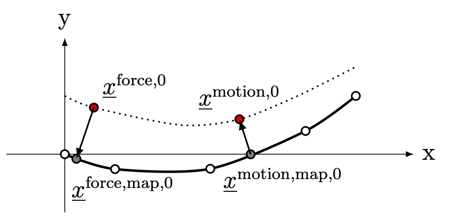
\[\begin{split}\begin{aligned} \underline{x}^\mathrm{force-con}_i &= -\underline{x}^{\mathrm{force},\mathrm{r}}_i + \underline{x}_i^{\mathrm{force},\mathrm{map},\mathrm{r}}, \qquad i \in \{ 1, \ldots, n^\mathrm{force} \} \\ \underline{x}^\mathrm{motion-con}_j &= \underline{x}_j^{\mathrm{motion},\mathrm{r}} - \underline{x}^{\mathrm{motion},\mathrm{map},\mathrm{r}}_j, \qquad j \in \{ 1, \ldots, n^\mathrm{motion} \} \end{aligned}\end{split}\]

6 Schematic of mapping between a 5-node beam element and fluid force-transfer and motion-transfer nodes.

Coupling in time

Overview

An Kynema goal is to provide an API that facilitates robust and accurate coupling with fluid-dynamics codes, like those in the ExaWind suite. Kynema needs to provide data to the fluid solver at the “right” time and place. In our approach, we assume that Kynema and the fluid solver are operating on a shared timeline. However, the structural time integration scheme is typically different than that of the fluid solver, and the codes may be using different time step sizes. For example, accuracy or stability requirements may require \(\Delta t^\mathrm{st} < \Delta t^\mathrm{fl}\), or vice versa, where \(\Delta t^\mathrm{st}\) and \(\Delta t^\mathrm{fl}\) are the structure and fluid time steps, respectively. In the following, \(\Delta t^{n+1}\) is the FSI timestep for data sharing between codes such that \(t^{n+1} = t^{n} + \Delta t^{n+1}\), and we require that \(\Delta t^\mathrm{fluid} = A \Delta t^\mathrm{structure}\) \(A\ge 1\) is a positive integer, and \(\Delta t^{n+1}\) is taken equal to \(\Delta t^\mathrm{fluid}\).

Depending on the fluid solver, Kynema output may be required at \(t^n\) (e.g., fluid solver is explicit), \(t^{n+1/2}\) (e.g., fluid solver is Crank-Nicolson), or \(t^{n+1}\) (e.g., fluid solver is backwards Euler). For example, the Nalu-Wind CFD code uses a backwards Euler time integration scheme and AMR-Wind uses a Crank-Nicolson-like solver; these two CFD codes are our primary targets for coupling.

Assume we know the following states at time \(t^n\), which are the data being transferred between the fluid and structure (see Eq. (14)):

\[\begin{aligned} \underline{f}_\ell^{n-1} \in \mathbb{R}^3, \, \underline{m}_\ell^{n-1} \in \mathbb{R}^3, \, \underline{q}_\ell^{n-1} \in \mathbb{R}^7,\, \underline{v}_\ell^{n-1} \in \mathbb{R}^6, \qquad \ell\in \{1,\ldots,P\} \end{aligned}\]

\[\underline{f}_\ell^n \in \mathbb{R}^3, \, \underline{m}_\ell^n \in \mathbb{R}^3, \, \underline{q}_\ell^n \in \mathbb{R}^7,\, \underline{v}_\ell^n \in \mathbb{R}^6, \qquad \ell\in \{1,\ldots,P\}\]

If we are coupling to AMR-Wind for actuator-line type simulations, simulations are facilitated if we also have the following data, which are the forces at the fluid nodes (for actuator-line simulations, those “nodes” are the aerodynamic centers) (see Force and Moment transfer: Fluid to structure):

\[\underline{f}_i^{\mathrm{fl},n} \in \mathbb{R}^3, \underline{f}_i^{\mathrm{fl},n-1} \in \mathbb{R}^3, \quad \forall i \in \{1, \ldots, n^\mathrm{fl} \}\]

The following describes the order of operations for the Kynema FSI API. It is “serial” in that the fluid and structure solvers are updated sequentially and not concurrently.

FSI Algorithm: Actuator-line CFD (AMR-Wind)

In the following approach, we assume that the fluid solver, e.g., AMR-Wind, needs positions and forces at the half step.

Step 1: Predict with first-order extrapolation the fluid forces and moments on structure nodes and forces at aerodynamic centers at \(t^{n+1}\):

\[\begin{split} \underline{f}_i^{n+1} \approx \underline{f}_i^{n} + \frac{\Delta t^{n+1}}{\Delta t^n} \left( \underline{f}^{n}_i - \underline{f}^{n-1}_i \right)\\ \underline{m}_i^{n+1} \approx \underline{m}_i^{n} + \frac{\Delta t^{n+1}}{\Delta t^n} \left( \underline{m}^{n}_i - \underline{m}^{n-1}_i \right)\\ \forall i \in \{1,\ldots,P\}\end{split}\]

\[\begin{split} \underline{f}_j^{\mathrm{fl},n+1} \approx \underline{f}_j^{\mathrm{fl},n} + \frac{\Delta t^{n+1}}{\Delta t^n} \left( \underline{f}^{\mathrm{fl},n}_j - \underline{f}^{\mathrm{fl},n-1}_j \right)\\ \forall j \in \{1,\ldots,n^\mathrm{force}\}\end{split}\]

Note: We do not need the moment at the aerodynamic centers at this time.

Step 2: Advance the Kynema solution to \(t^{n+1} = t^n + \Delta t^{n+1}\), using nodal forces (either predicted in Step 1 or, if iterating, solved in Step 7) at \(t^{n+1}\). In the case that the structure uses substeps, use force values linearly interpolated between those at \(t^{n+1}\) and \(t^n\).

Step 3: Update the locations and velocities of the aerodynamic centers; i.e., calculate \(\underline{x}^{\mathrm{fl},n+1}_j\) and \(\dot{\underline{u}}^{\mathrm{fl},n+1}_j\) following Motion transfer: Structure to fluid nodes

Step 4: Interpolate from \(t^{n}\) and \(t^{n+1}\) the positions of the aerodynamic centers and the forces at those locations to \(t^{n+1/2}\):

\[\begin{split}\underline{x}_j^{\mathrm{fl},n+1/2} = \frac{1}{2} \left( \underline{x}_j^{\mathrm{fl},n} + \underline{x}_j^{\mathrm{fl},n+1} \right) \\ \underline{f}_j^{\mathrm{fl},n+1/2} = \frac{1}{2} \left( \underline{f}_j^{\mathrm{fl},n} + \underline{f}_j^{\mathrm{fl},n+1} \right) \\ \forall j \in \{1,\ldots,n^\mathrm{force}\}\end{split}\]

Step 5: Advance the CFD solution to \(t^{n+1}\) using forces located at interpolated positions of aerodynamic centers at \(t^{n+1/2}\) (from Step 4).

Step 6: At \(t^{n+1}\) calculate the fluid forces and moments (see Blade-element aerodynamics solver) at the aerodynamic centers (locations calculated in Step 3) and based on the aerodynamic center velocities calculated in Step 3 and the CFD fluid velocities.

Yields \(\underline{f}_j^{\mathrm{fl},n+1}\) and \(\underline{m}_j^{\mathrm{fl},n+1}\) for all \(j \in \{1, \ldots, n^\mathrm{force}\}\)

Step 7: At \(t^{n+1}\) calculate the fluid forces and moments at structure nodes following Force and Moment transfer: Fluid to structure based on forces and moments calculated in Step 6.

Yields \(\underline{f}_\ell^{n+1}\) and \(\underline{m}_\ell^{n+1}\) for all \(\ell \in \{1, \ldots, P\}\)

Step 8: Either accept completion of time advance, or go back to Step 2 and repeat with latest forces and positions. Note that one might to choose to only recalculate the structure solve, but that would potentially create a discrepancy between fluid and structure locations at \(t^{n+1}\).

FSI Algorithm: geometry-resolved CFD (Nalu-Wind)

Step 1: Predict/extrapolate the fluid forces at strcture nodes \(t^{n+1} = t^n + \Delta t^{n+1}\)

\[\begin{split}\begin{aligned} \underline{f}_i^{n+1} \approx \underline{f}_i^{n} + \frac{\Delta t^{n+1}}{\Delta t^n} \left( \underline{f}^{n}_i - \underline{f}^{n-1}_i \right)\\ \underline{m}_i^{n+1} \approx \underline{m}_i^{n} + \frac{\Delta t^{n+1}}{\Delta t^n} \left( \underline{m}^{n}_i - \underline{m}^{n-1}_i \right) \end{aligned}\end{split}\]

Step 2: Advance the Kynema solution to \(t^{n+1} = t^n + \Delta t^{n+1}\), using forces predicted/solved at \(t^{n+1}\). In the case that the structure uses substeps, use force values linearly interpolated between those at \(t^{n+1}\) and \(t^n\).

Step 3: Based on the nodal values at \(t^{n}\) and \(t^{n+1}\), calculate the associated positions and velocities of the fluid nodes at \(t^{n+1}\) following Motion transfer: Structure to fluid nodes.

Step 4: Advance the fluid solver based on motion calculated by the structural solver in Step 2.

Step 5: Update the fluid forces at structure nodes following Force and Moment transfer: Fluid to structure.

Step 6: Either accept completion of time advance, or go back to Step 2 and repeat with latest fluid forces from Step 3. Note that one might to choose to only recalculate the structure solve, but that would potentially create a discrepancy between fluid and structure locations at \(t^{n+1}\).

Motion transfer: Structure to fluid nodes

As the first step, generalized displacements and velocities are calculated at the mapped locations on the structure:

\[\begin{split}\begin{aligned} \underline{q}_j^{\mathrm{motion},\mathrm{map}} = \begin{bmatrix} \underline{u}_j^{\mathrm{motion},\mathrm{map}} \\ \widehat{q}_j^{\mathrm{motion},\mathrm{map}} \end{bmatrix} \qquad \underline{v}_j^{\mathrm{motion},\mathrm{map}} = \begin{bmatrix} \underline{\dot{u}}_j^{\mathrm{motion},\mathrm{map}} \\ \underline{\omega}_j^{\mathrm{motion},\mathrm{map}} \end{bmatrix}, \qquad j \in \{ 1, \ldots, n^\mathrm{motion} \} \end{aligned}\end{split}\]

where

\[\begin{split}\begin{aligned} \underline{u}_j^{\mathrm{motion},\mathrm{map}} = \sum_{\ell=1}^P \phi_\ell \left(\xi_j^{\mathrm{motion},\mathrm{map}} \right) \underline{u}_\ell \\ \widehat{q}^{\mathrm{motion},\mathrm{map}}_j = \frac{ \sum_{\ell=1}^{P} \phi_\ell\left(\xi_j^{\mathrm{motion},\mathrm{map}} \right) \widehat{q}_\ell} {|| \sum_{\ell=1}^{P} \phi_\ell\left(\xi_j^{\mathrm{motion},\mathrm{map}} \right) \widehat{q}_\ell ||} \\ \underline{v}_j^{\mathrm{motion},\mathrm{map}} = \sum_{\ell=1}^P \phi_\ell \left(\xi_j^{\mathrm{motion},\mathrm{map}} \right) \underline{v}_\ell \\ \end{aligned}\end{split}\]

The current position of the fluid nodes (in global/inertial coordinates) is

\[\begin{aligned} \underline{x}_j^\mathrm{fl} = \underline{x}_j^{\mathrm{motion},\mathrm{r}} + \underline{u}_j^{\mathrm{motion},\mathrm{map}} + \left[ \underline{\underline{R}}(\widehat{q}_j^{\mathrm{motion},\mathrm{map}}) - \underline{\underline{I}} \right] \underline{x}^\mathrm{motion-con}_j, \qquad j \in \{ 1, \ldots, n^\mathrm{motion} \} \end{aligned}\]

and the current velocity of the fluid nodes is

\[\begin{aligned} \dot{\underline{u}}_j^\mathrm{fl} = \dot{\underline{u}}_j^{\mathrm{motion},\mathrm{map}} + \underline{\omega}^{\mathrm{motion},\mathrm{map}}_j \times \left[\underline{\underline{R}}(\underline{\widehat{q}}_j^{\mathrm{motion},\mathrm{map}})\underline{x}^\mathrm{motion-con}_j\right],\, \qquad j \in \{ 1, \ldots, n^\mathrm{motion} \} \end{aligned}\]

These are passed to the fluid solver.

Force and Moment transfer: Fluid to structure

We have a set of \(n^\mathrm{force}\) forces and moments, \(\underline{f}^\mathrm{force}_i\) and \(\underline{m}^\mathrm{force}_i\), with reference locations \(\underline{x}_i^{\mathrm{force},\mathrm{r}}\).

We need the orientations:

\[\begin{aligned} \widehat{q}^{\mathrm{force},\mathrm{map}}_j = \frac{ \sum_{\ell=1}^{P} \phi_\ell\left(\xi_j^{\mathrm{force},\mathrm{map}} \right) \widehat{q}_\ell} {|| \sum_{\ell=1}^{P} \phi_\ell\left(\xi_j^{\mathrm{force},\mathrm{map}} \right) \widehat{q}_\ell ||} \,, \qquad j \in \{ 1, \ldots, n^\mathrm{force} \} \end{aligned}\]

Nodal forces (at \(P\) nodes) are

\[\begin{aligned} \underline{f}_\ell = \sum_{j=1}^{n^\mathrm{force}} \phi_\ell(\xi^{\mathrm{force},\mathrm{map}}_j) \underline{f}^\mathrm{force}_j, \qquad \ell \in \{ 1, \ldots, P \} \label{eq:force} \end{aligned}\]

Nodal moments (at \(P\) nodes) are

\[\begin{aligned} \underline{m}_\ell = \sum_{j=1}^{n^\mathrm{force}} \phi_\ell(\xi^{\mathrm{force},\mathrm{map}}_j) \left[\underline{f}^\mathrm{force}_j \times \left( \underline{\underline{R}}(\widehat{q}^{\mathrm{force},\mathrm{map}}_j) \underline{x}^\mathrm{force-con}_j\right) + \underline{m}^\mathrm{force}_j\right], \qquad \ell \in \{ 1, \ldots, P \} \label{eq:moment} \end{aligned}\]