Beam reference lines and reference configuration
The use of LSFEs as our beam spatial discretization presents opportunities and challenges for the geometric representation of slender structures like turbine blades. Turbine blades can be curved, swept, and/or twisted along their length. In this section we describe how beams are user defined and how the beams are discretized in the reference configuration.
Kynema beams are assumed to be defined as a set of points in the global coordinate system \((\widehat{x}^\mathrm{g}, \widehat{y}^\mathrm{g},\widehat{z}^\mathrm{g})\) with the blade root positioned on the \(\widehat{x}^\mathrm{g}\) axis and oriented such that the pitch axis, or its primary-length direction, is pointing in the \(x\) direction. For turbine blades, the \(y\) direction is the direction of the trailing edge and defines a zero pitch/twist. Note that this differs from the standard turbine-blade definition, which can be easily rotated into our system.
The user must provide \(n^\mathrm{geom} \ge 2\) points defining the reference line with the data \((\eta_i^\mathrm{geom},\underline{x}_i^\mathrm{geom},\tau_i^\mathrm{geom})\), \(i \in \{ 1, 2, \ldots, n^\mathrm{geom}\}\), where \(\eta_i^\mathrm{geom}\in[0,1]\) defines the nondimensional position along the beam reference line where the associated reference line position is \(\underline{x}_i^\mathrm{geom} \in \mathbb{R}^3\) and twist about the reference line is \(\tau_i^\mathrm{geom}\). Note that Kynema convention requires that \(\underline{x}_1^\mathrm{geom} = (x_1, 0, 0)^T\).
The user must also provide (through quadrature input choices) the \(n^Q\) quadrature locations \(\xi_k^Q \in [-1,1]\) along the reference axis.
Finally, the user must provide the translation and rotation, \(\underline{u}^\mathrm{move}\) and \(\underline{\underline{R}}^\mathrm{move}\), respectively, that moves the beam from its setup postion/orientation to its reference position/orientation. \(\underline{x}^\mathrm{r}\) and \(\underline{\underline{R}}^\mathrm{r}\), respectively. In other words, each beam is defined in the global system and it is then translated and rotated into its reference position. While we present a single \(\underline{u}^\mathrm{move}\) and a single \(\underline{\underline{R}}^\mathrm{move}\), in practice those are implemented in multiple steps.
Our approach is to represent the geometry with a single spectral element with relatively few points, which we describe here. Given \(n^\mathrm{geom}\) points describing the beam as above, we wish to represent that beam with a \(P\)-point Legendre spectral finite element, where \(P\) is a user input.
We first perform a least-squares fit to the data using a LSFE polynomial with \(\mathrm{min}(P,n^\mathrm{geom})\) points, where the endpoints of the fitting polynomial are constrained to coincide with the reference data at \(\eta_1^\mathrm{geom}\) and \(\eta^\mathrm{geom}_{n^\mathrm{geom}}\). If \(P \le n^\mathrm{geom}\), that fit defines the \(P\) nodal locations of the LSFE. If \(P > n^\mathrm{geom}\), then a new LSFE is constructed with \(P\)-nodes that lie on the lower-order \(n^\mathrm{geom}\)-point least-squares fit. The result are nodal values \(\underline{x}^\mathrm{fit}_\ell \in \mathbb{R}^3\), for \(\ell \in \{1, \ldots, P\}\). The geometry of the reference line is given (in the element natural coordinates) as
for \(\xi\in[-1,1]\).
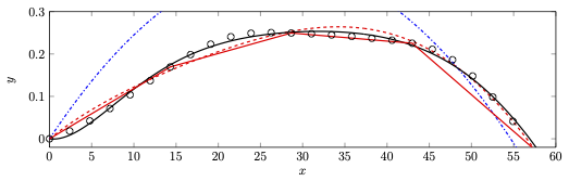
Figure 1 shows the results of the fitting process for the IEA 15-MW reference turbine, which is defined by 50 points. Shown are LSFE fits with 3, 7, and 10 nodes. Clearly the 10-node fit provides an excellent geometric approximation of the discrete data. For reference, also shown is 10-node representation with linear segments, which emphasizes the advantage of the LSFE representation for a given number of nodes.
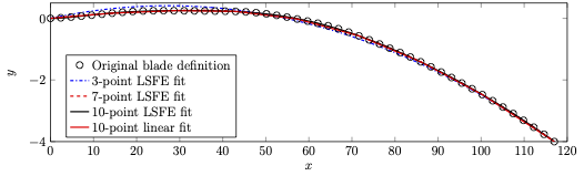
1 Discrete representation of the IEA 15-MW reference-turbine blade reference line with 50 points, and four continuous-function representations of the beam reference line.
A beam’s reference line also requires the definition of its orientation. We construct the orientation from the LSFE line as follows:
Calculate the unit tangent at each LSFE node:
\[\begin{aligned} \widehat{t}^{\mathrm{fit}}_i = \sum_{\ell=1}^P \underline{x}^\mathrm{fit}_\ell \left . \frac{\partial \phi_\ell}{\partial \xi}\right|_{\xi=\xi_i} / \left \Vert\sum_{i=1}^P \underline{x}^\mathrm{fit}_i \left . \frac{\partial \phi_i}{\partial \xi}\right|_{\xi=\xi_i} \right\Vert , \quad \forall i \in \{1, \ldots, P\} \end{aligned}\]At each LSFE node, calculate a unit vector, \(\widehat{n}^\mathrm{fit}_i\), normal to \(\widehat{t}^\mathrm{fit}_i\) with the additional requirement that it lies in the local \(\widehat{x}^\mathrm{g}-\widehat{y}^\mathrm{g}\) plane, i.e., \(\widehat{n}^\mathrm{fit}_i = (n_1^\mathrm{fit},n_2^\mathrm{fit}, 0 )\) with the requirements \(\left|\widehat{n}^\mathrm{fit}_i \right | = 1\) and \(\widehat{n}^\mathrm{fit}_i \cdot \widehat{t}^\mathrm{fit}_i = 0\).
The binormal vector is then given by \(\underline{b}^\mathrm{fit}_i = \widetilde{t^\mathrm{fit}_i} \underline{n}^\mathrm{fit}_i\).
The orientation at node \(i\) is given by
\[\begin{aligned} \underline{\underline{R}}^\mathrm{fit}_i = \begin{bmatrix} \widehat{t}^\mathrm{fit}_i \,\, \widehat{n}^\mathrm{fit}_i \,\, \widehat{b}^\mathrm{fit}_i \end{bmatrix} ,\, \forall i \in \{1, \ldots, P\} \end{aligned}\]which has the associated quaternions \(\widehat{q}_i^\mathrm{fit}\).
Nodal positions in the reference position, given \(\underline{u}^\mathrm{move}\) and \(\underline{\underline{R}}^\mathrm{move}\), are calculated as
\[\begin{aligned} \underline{x}^\mathrm{r}_i = \underline{x}^\mathrm{fit}_i + \underline{u}^\mathrm{move} +\underline{\underline{R}}^\mathrm{move} \left(\underline{x}^\mathrm{fit}_i- \underline{x}^\mathrm{fit}_1\right) \quad \forall i \in \{1, \ldots, P \} \end{aligned}\]Nodal orientations are calculated as
\[\begin{aligned} \underline{\underline{R}}^\mathrm{r}_i = \underline{\underline{R}}^\mathrm{move} \underline{R}^\mathrm{fit}_i ,\quad \forall i \in \{1, \ldots, P \} \end{aligned}\]which has the associated quaternions \(\widehat{q}_i^\mathrm{r}\).
We also require the reference orientations at quadrature points, \(\xi^\mathrm{Q}_k\), which are calculated and stored as quaternions:
\[\begin{aligned} \widehat{q}^{\mathrm{r,Q}}_k = \sum_{\ell=1}^P \widehat{q}^\mathrm{r}_\ell \phi_\ell\left(\xi_k^\mathrm{Q}\right) / \left \Vert\sum_{\ell=1}^P \widehat{q}^\mathrm{r}_\ell \phi_\ell\left(\xi_k^\mathrm{Q} \right) \right \Vert , \quad \forall k \in \{1, \ldots, n^\mathrm{Q}\} \end{aligned}\]Finally, regarding the user defined twist, that is applied at initialization to the sectional material matrices, e.g., for the mass matrices:
\[\begin{split}\begin{bmatrix} \underline{\underline{R}}(\tau_k) & \underline{\underline{0}} \\ \underline{\underline{0}} & \underline{\underline{R}}(\tau_k) \end{bmatrix} \underline{\underline{M}}_k^* \begin{bmatrix} \underline{\underline{R}}(\tau_k) & \underline{\underline{0}} \\ \underline{\underline{0}} & \underline{\underline{R}}(\tau_k) \end{bmatrix}^T \rightarrow \underline{\underline{M}}_k^*\end{split}\]where \(\underline{\underline{M}}_k^*\) and \(\tau_k\) are linearly interpolated mass matrix and twist (at each quadrature point), respectively, from nearest neighbors, and
\[\begin{split}\underline{\underline{R}}(\tau) = \begin{bmatrix} 1 & 0 & 0 \\ 0 & \cos(\tau) & - \sin(\tau) \\ 0 & \sin(\tau) & \cos(\tau) \end{bmatrix}\end{split}\]